
One small 8-pin chip sits at the heart of almost every analog circuit you will ever meet: the microphone preamplifier, the temperature sensor, the audio mixer, the power supply error amplifier, and the comparator that watches a battery voltage. It is the operational amplifier — the op-amp — and it is the most versatile building block in electronics. Give it two resistors and it becomes a precise amplifier. Add a capacitor and it integrates, differentiates, or filters. Remove the feedback entirely and it becomes a comparator.
This guide explains what an op-amp is, how it works inside, the two golden rules that let you analyze any op-amp circuit, the inverting and non-inverting configurations with worked examples, the real-world limits that catch beginners out, and where op-amps are used. If you need the background first, our guides to semiconductors and transistors explain the silicon the op-amp is built from.
What Is an Op-Amp?
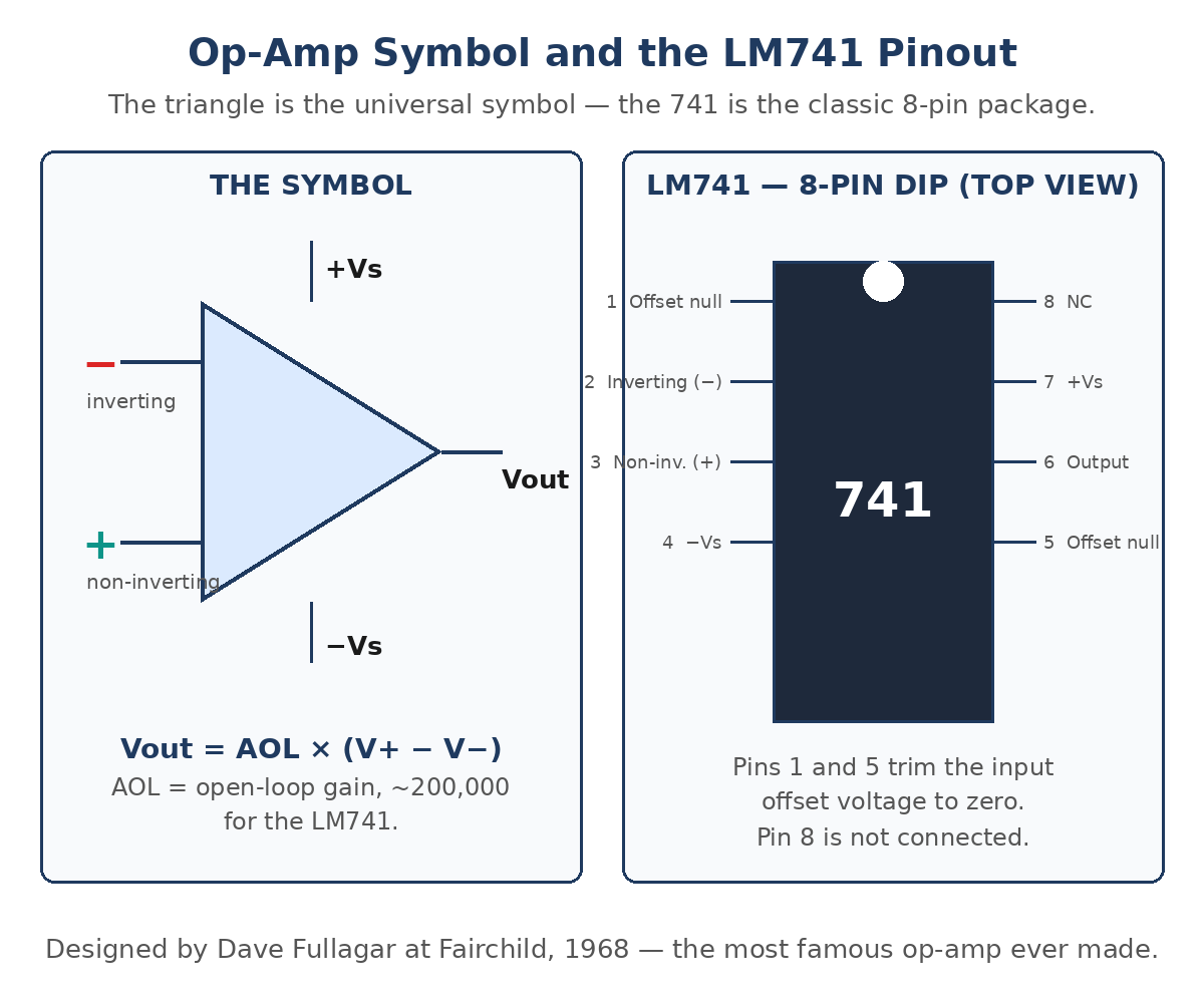
An operational amplifier (op-amp) is a high-gain differential voltage amplifier with two inputs and one output. The two inputs are the inverting input (−) and the non-inverting input (+). The output voltage is the difference between the two input voltages, multiplied by a very large gain: Vout = AOL × (V+ − V−), where AOL is the open-loop gain. For the classic LM741, AOL is about 200,000 — so a 10 µV difference between the inputs would already drive the output to 2 V.
The name comes from the 1960s, when these amplifiers were used in analog computers to perform mathematical operations — addition, subtraction, integration, differentiation — on electrical signals. The first op-amp offered to the public was Fairchild’s µA702 in 1963, but the device that made the op-amp famous was the µA741, designed by Dave Fullagar at Fairchild Semiconductor in 1968. It was the first op-amp with internal frequency compensation, so it was stable without external components, and it is still manufactured and taught today. Inside the little 8-pin package are about 20 transistors, arranged in stages: a differential input stage, a gain stage, and a push-pull output stage.
The Ideal Op-Amp and the Two Golden Rules
A real op-amp is a complicated circuit, but for almost all analysis you only need the ideal model. An ideal op-amp has infinite open-loop gain, infinite input impedance, zero output impedance, infinite bandwidth, and zero input offset voltage. No real device achieves any of those, but the ideal model is close enough to design with — and the gap between ideal and real is exactly what the limits section below is about.
When an op-amp is wired with negative feedback — that is, when part of the output is fed back to the inverting input — the ideal model collapses into two golden rules that solve nearly every linear op-amp circuit:
- Rule 1 — no input current: no current flows into either input terminal, because the ideal input impedance is infinite. Every milliamp that flows through the input resistor must therefore continue through the feedback resistor.
- Rule 2 — the virtual short: the voltage difference between the two inputs is zero (V+ = V−), because the enormous open-loop gain forces any difference toward zero when feedback is present. The inputs behave as if they were shorted together for voltage purposes, even though no current flows between them.
Both rules only hold while the op-amp is in its linear region — with negative feedback, and with the output not saturated against a supply rail. Keep those conditions in mind and the rules will carry you through every configuration below.
The Inverting Amplifier
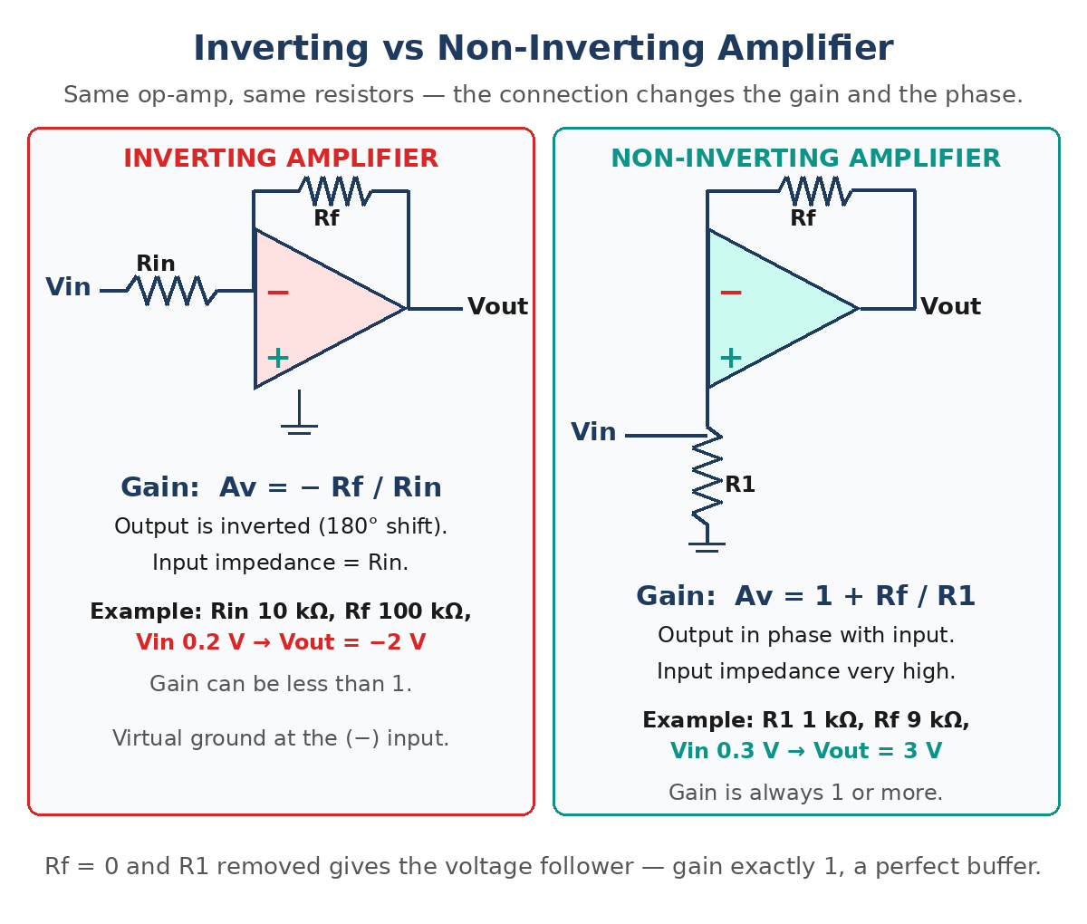
In the inverting configuration, the input signal drives the inverting (−) terminal through a resistor Rin, a feedback resistor Rf connects the output back to the same terminal, and the non-inverting (+) terminal is grounded. By Rule 2, the (−) terminal sits at the same voltage as the (+) terminal — 0 V. That node is called a virtual ground: it is held at zero volts by feedback, even though it is not actually connected to ground.
By Rule 1, no current enters the op-amp, so the current through Rin must all flow through Rf. The current through Rin is Vin / Rin, and the voltage drop across Rf is that current times Rf, so the output is Vout = −(Rf / Rin) × Vin. The voltage gain is therefore Av = −Rf / Rin. The minus sign means the output is inverted — 180° out of phase with the input. The input impedance the source sees is just Rin, because the source drives a resistor whose far end is held at virtual ground.
Worked example: Rin = 10 kΩ, Rf = 100 kΩ, Vin = 0.2 V. The gain is −100 / 10 = −10, so Vout = −10 × 0.2 = −2 V. The signal is amplified ten times and flipped in polarity. Note that the gain can be less than 1 — choose Rf smaller than Rin and the circuit attenuates instead of amplifying, which is sometimes exactly what you want.
The Non-Inverting Amplifier
In the non-inverting configuration, the input signal goes directly to the (+) terminal, and the feedback network — Rf from the output to the (−) terminal and R1 from the (−) terminal to ground — forms a voltage divider. By Rule 2, V− = V+ = Vin, and the divider sets V− = Vout × R1 / (R1 + Rf). Rearranging gives Av = 1 + Rf / R1. The output is in phase with the input, and the gain is always 1 or more — it can never attenuate.
The great advantage of this circuit is its input impedance: because the signal feeds directly into the op-amp’s (+) input, the input impedance is the op-amp’s own — megohms or more — so it barely loads the source at all. That is why the non-inverting amplifier is the right choice for weak, high-impedance sources such as sensors and microphones. The resistor values set the gain, and nothing else does — the op-amp’s own gain never appears in the formula, which is the whole point of negative feedback.
Worked example: R1 = 1 kΩ, Rf = 9 kΩ, Vin = 0.3 V. The gain is 1 + 9 / 1 = 10, so Vout = 10 × 0.3 = 3 V, in phase with the input. Compare that with the inverting example above: the same resistor ratio gives +10 instead of −10, and the input draws essentially no current.
The Voltage Follower (Unity-Gain Buffer)
The voltage follower is a special case of the non-inverting amplifier: set Rf = 0 (a wire from output straight back to the (−) input) and remove R1, and the gain formula gives Av = 1 + 0 = 1. The output voltage exactly tracks the input voltage — no amplification at all. So why build a circuit with a gain of 1? Because it is a buffer: it has the op-amp’s huge input impedance and tiny output impedance, so it can take a weak signal that would collapse under any load and drive a heavy load with it. Voltage followers sit between sensors and analog-to-digital converters, between signal sources and long cables, and anywhere else a signal needs to be copied without being loaded down.
Other Op-Amp Configurations
Once you have the two golden rules, the rest of the op-amp family follows by changing what sits in the feedback network:
- Summing amplifier: several inputs, each through its own resistor, into the inverting terminal. The output is the weighted sum of the inputs — the heart of an audio mixer. Vout = −Rf × (V1/R1 + V2/R2 + …).
- Differential amplifier: inputs applied to both terminals through matched resistor dividers. The output is proportional to the difference between the two inputs and rejects any voltage common to both — the basis of instrumentation amplifiers and sensor front ends.
- Integrator: a capacitor in the feedback path instead of a resistor. The output is the time integral of the input — the output ramps up as long as the input is positive. Used in waveform generators and control loops.
- Differentiator: a capacitor at the input and a resistor in the feedback path. The output is proportional to the rate of change of the input — useful for edge detection, but noisy in practice.
- Comparator: no feedback at all. The enormous open-loop gain slams the output to one supply rail or the other depending on which input is higher — a one-bit analog-to-digital converter. Add a little positive feedback and it becomes a Schmitt trigger, with hysteresis that stops the output chattering on noisy signals.
- Active filter: resistors and capacitors arranged so the op-amp passes some frequencies and blocks others — low-pass, high-pass, and band-pass filters for audio and signal conditioning.
Real-World Limits: What the Ideal Model Hides
Real op-amps break the ideal rules in specific, predictable ways, and knowing them is what separates a circuit that works on paper from one that works on the bench. Here are the LM741’s numbers as a reference — modern op-amps are better on every line, but the concepts are the same:
| Parameter | Ideal Op-Amp | LM741 (Typical) | What It Means in Practice |
|---|---|---|---|
| Open-loop gain (AOL) | Infinite | 200,000 (106 dB) | Closed-loop gain is set by resistors, not by AOL |
| Input impedance | Infinite | 2 MΩ | Draws a small bias current (~80 nA) |
| Output impedance | Zero | ~75 Ω | Feedback lowers it to milliohms in closed loop |
| Gain-bandwidth product | Infinite | 1 MHz | Gain × bandwidth is constant |
| Slew rate | Infinite | 0.5 V/µs | Output cannot change faster than this |
| Input offset voltage | Zero | 1–6 mV | A small error voltage; trimmed with pins 1 and 5 |
| Supply voltage | Any | ±5 V to ±18 V (typical ±15 V) | Output cannot exceed the supplies |
| Output swing | Unlimited | About ±13 V on ±15 V supplies | Not rail-to-rail — it saturates ~2 V from each rail |
Two limits catch beginners most often. The first is saturation: an op-amp cannot output more than its supply allows. Take the non-inverting example above (gain 10) and apply Vin = 1.5 V — the formula says 15 V, but on ±15 V supplies the 741 clips at about ±13 V, and on ±12 V supplies at about ±10–11 V. The output flattens, the signal distorts, and the gain formulas stop applying. Always check that |Vout| stays inside the supply rails before trusting the math.
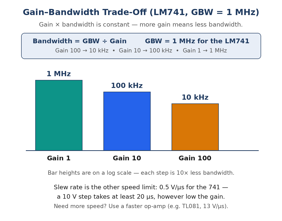
The second is the gain–bandwidth trade-off: gain times bandwidth is constant, equal to the gain-bandwidth product (1 MHz for the 741). Set a gain of 100 and the circuit only works cleanly up to 10 kHz; set a gain of 10 and it works to 100 kHz; set a gain of 1 and it works to 1 MHz. And the slew rate (0.5 V/µs for the 741) limits large fast signals separately: a 10 V step takes at least 20 µs, however low the gain. If you need more speed, choose a faster op-amp — the TL081, for example, manages 13 V/µs.
Where Op-Amps Are Used
- Audio: microphone preamplifiers, mixers, tone controls, and headphone drivers — the non-inverting amplifier and the summing amplifier in daily use.
- Sensors: amplifying tiny signals from thermocouples, strain gauges, and photodiodes, usually with an instrumentation amplifier built from three op-amps.
- Signal conditioning: buffering, filtering, and level-shifting signals before they reach an analog-to-digital converter.
- Power supplies: the error amplifier inside a voltage regulator compares the output with a reference and corrects it — a voltage follower with a mission.
- Comparators and timers: threshold detection, zero-crossing detection, and the classic 555 timer’s internal comparators.
- Oscillators and waveform generators: sine, square, and triangle waves built from integrators and Schmitt triggers.
Frequently Asked Questions
What does an op-amp do?
An op-amp amplifies the voltage difference between its two inputs by a very large gain. Wrapped in a feedback network of resistors and capacitors, that raw gain becomes precise, predictable circuits: amplifiers, buffers, filters, integrators, and comparators.
What is the difference between an inverting and a non-inverting amplifier?
The inverting amplifier feeds the signal into the (−) input through a resistor: gain is −Rf / Rin, the output is flipped 180°, and the input impedance equals Rin. The non-inverting amplifier feeds the signal straight into the (+) input: gain is 1 + Rf / R1, the output stays in phase, the gain is always 1 or more, and the input impedance is very high.
What is a virtual ground?
In an inverting amplifier, the (−) input node is held at 0 V by negative feedback even though it is not connected to ground — because the (+) input is grounded and the virtual-short rule forces V− = V+. It is called virtual because no current can actually flow into that ground; it is a voltage condition, not a connection.
Why is the LM741 still taught if it is old?
Because it is the simplest op-amp to learn on: an 8-pin package, a ±15 V supply, a 1 MHz gain-bandwidth product, and a 0.5 V/µs slew rate that makes its limits easy to see. Everything you learn on a 741 — the golden rules, the gain formulas, saturation, and the gain-bandwidth trade-off — applies directly to modern op-amps, which are simply better on every specification.
Can an op-amp work on a single supply?
Yes, with care. A standard op-amp like the 741 needs its inputs and output to stay between the two supply rails, so on a single +12 V supply you normally bias the (+) input to a mid-rail reference (6 V) so the signal can swing both ways. Single-supply and rail-to-rail op-amps are designed for exactly this job and are the usual choice for battery-powered circuits.
Conclusion
The op-amp earns its place in almost every analog circuit because it turns one hard problem — building a precise amplifier — into an easy one: pick two resistors and let negative feedback do the rest. The two golden rules (no input current, and the virtual short) give you the inverting gain −Rf / Rin and the non-inverting gain 1 + Rf / R1, and from those two formulas come buffers, summers, filters, and integrators. The real world adds its limits — saturation at the supply rails, the 1 MHz gain-bandwidth trade-off, and the 0.5 V/µs slew rate of the classic 741 — but those limits are predictable, and choosing a modern op-amp moves every one of them. Start with the 741, learn the rules, and you can read any op-amp circuit you meet. For a structured study guide with more derivations and worked examples, see Operational Amplifiers on Expert Study Guides.