
Introduction
Picture an electrician standing in front of a factory distribution panel. Two transformers feed the board, dozens of breakers branch off in every direction, and a fault somewhere is tripping the main breaker. The simple series-and-parallel rules from basic training are not enough here — the circuit is a tangled network of loops and junctions. How do you calculate the current in any single branch?
The answer comes from two elegant rules published in 1845 by German physicist Gustav Kirchhoff. Kirchhoff’s laws let you analyze any electrical network, no matter how complicated, by applying just two ideas: charge cannot pile up at a junction, and energy cannot appear or vanish around a loop.
In this guide, you will learn what Kirchhoff’s laws state, how their working principle operates through simple water and hiking analogies, the difference between KCL and KVL, and step-by-step worked examples. You will also discover Kirchhoff’s laws applications in real engineering, their advantages and disadvantages, and the mistakes that trap most beginners.
What Are Kirchhoff’s Laws?
Kirchhoff’s laws are two rules that describe how current and voltage behave in electrical networks:
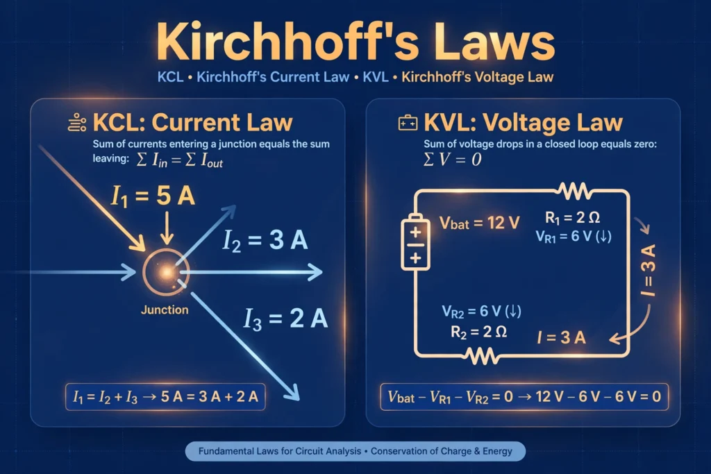
Kirchhoff’s Current Law (KCL): At any junction (node) in a circuit, the sum of currents entering the junction equals the sum of currents leaving it. In equation form, the algebraic sum of all currents at a node is zero (ΣI = 0). This is really the law of conservation of electric charge — charge cannot accumulate at a point.
Kirchhoff’s Voltage Law (KVL): Around any closed loop in a circuit, the algebraic sum of all voltages is zero (ΣV = 0). In plain words, if you walk around a loop and add up every voltage rise and drop, you end exactly where you started. This is the law of conservation of energy.
Practical example: at a junction, 5 amps flow in through one wire, while 2 amps and 3 amps flow out through two other wires — 5 = 2 + 3, so KCL is satisfied. In a loop with a 12 V battery and three resistors dropping 7 V, 3 V, and 2 V, the drops add to 12 V, matching the rise — KVL is satisfied.
Working Principle
The working principle of Kirchhoff’s laws becomes obvious with two everyday analogies:
- KCL is like water pipes joining. If three pipes meet at a junction and 10 litres per second flow in through one pipe, exactly 10 litres per second must flow out through the other two combined. Water cannot pile up inside the joint — and electric charge cannot pile up at a node either.
- KVL is like a hill hike. If you climb 100 metres up and later walk back down to your starting point, your total height change is zero. Similarly, every voltage “climb” (rise across a battery) must be matched by voltage “descents” (drops across resistors) around any closed loop.
Here is the step-by-step method engineers use:
First, label every branch current with an arrow showing its assumed direction. Second, for KCL, write at each node: currents entering = currents leaving (or ΣI = 0, treating entering as positive and leaving as negative). Third, for KVL, walk around each loop and add voltage drops as positive when moving from + to − across a component, and voltage rises as negative — or use any consistent sign rule. Fourth, solve the resulting equations together. If a current comes out negative, your assumed arrow was simply backwards; the magnitude is still correct.
Types of Kirchhoff’s Laws
There are two laws, plus an important extension for AC circuits. Each deserves its own explanation:
Kirchhoff’s Current Law (KCL)
KCL applies at a node — any point where two or more branches meet. The rule ΣI = 0 means charge is conserved: electrons arrive exactly as fast as they leave. KCL is the basis of nodal analysis, the method of finding unknown node voltages. It works for DC and AC alike, and it is the reason a clamp meter around a healthy cable bundle reads zero — the outgoing and returning currents cancel.
Kirchhoff’s Voltage Law (KVL)
KVL applies around a loop (also called a mesh) — any closed path through the circuit. The rule ΣV = 0 means energy is conserved: the energy the source gives each charge is fully spent crossing the loads. KVL is the basis of mesh analysis, the method of finding unknown loop currents. Sign discipline matters here: pick one convention (for example, voltage drops positive in the walking direction) and never change it mid-problem.
The Difference Between KCL and KVL
The difference between KCL and KVL is simple once stated plainly: KCL is about current at a point and rests on the conservation of charge, while KVL is about voltage around a path and rests on the conservation of energy. KCL answers “where does the current go?” at junctions; KVL answers “do the voltages balance?” around loops. In real analysis the two are almost always used together — KCL at the nodes, KVL around the meshes — to fully solve a network.
Kirchhoff’s Laws in AC Circuits
Both laws work unchanged for alternating current, provided you use phasor quantities: currents and voltages become complex numbers with magnitude and phase angle. KCL still holds at every instant and for phasors; KVL still holds around every loop. This is how power-system engineers analyze entire national grids.
Main Components
To apply Kirchhoff’s laws, you need to recognize four circuit concepts — the “components” of the method itself:
Node (junction): a point where two or more branches connect. KCL is written here. A simple series circuit has no useful nodes; a parallel network has several.
Branch: a single path between two nodes, usually containing one or more components. Each branch carries one unknown current.
Loop (mesh): any closed path through branches. KVL is written here. A mesh is a loop with no other loops inside it.
Sign convention: the bookkeeping rule that makes the math work — for example, currents entering a node positive and leaving negative, or voltage drops positive when traversed from + to −. Consistency matters more than which choice you make.
Advantages
- Handles any network: no matter how tangled the circuit, KCL and KVL always give enough equations to solve it.
- Foundation of analysis: nodal and mesh analysis — the two standard professional methods — are built directly on these laws.
- Works for AC and DC: with phasors, the same laws analyze power systems and electronics alike.
- Fault-finding power: if measured branch currents violate KCL, you have found a leakage or fault path.
- Physically grounded: because they rest on conservation of charge and energy, they can never be “wrong” for lumped circuits.
- Scales with software: circuit simulators apply these laws thousands of times per second behind the scenes.
Disadvantages and Limitations
Kirchhoff’s laws are reliable, but they have honest limitations every student should know:
- Tedious by hand: a circuit with ten meshes needs ten simultaneous equations — practical only with software or patience.
- Lumped-element assumption: the laws assume components are concentrated at points. At very high frequencies or on long transmission lines, wires themselves store energy and the simple laws need extensions.
- Sign errors: the math is easy; keeping the + and − signs consistent is where most beginners fail.
- No component values: the laws relate voltages and currents but cannot tell you what resistor value to choose — Ohm’s law must join the work.
- Linear circuits preferred: with non-linear devices like transistors, the equations become much harder to solve directly.
Applications
Kirchhoff’s laws applications span from classroom to national power grids:
- Circuit design: every PCB and power supply is verified with nodal and mesh analysis before manufacturing.
- Fault finding: technicians compare measured branch currents against KCL — a mismatch reveals leakage, partial shorts, or earth faults.
- Power systems: load-flow studies of transmission networks are giant KCL/KVL problems solved by computers.
- Electronics: transistor biasing and amplifier analysis start with KVL loops and KCL nodes.
- Instrumentation: bridge circuits (like the Wheatstone bridge) are analyzed and balanced using KVL.
- Automotive electrics: tracing parasitic battery drains uses KCL thinking — all branch currents must add up.
Kirchhoff’s Laws Comparison
This table puts the two laws side by side so the difference is crystal clear:
| Feature | KCL (Current Law) | KVL (Voltage Law) |
|---|---|---|
| Applies to | A node (junction) | A closed loop (mesh) |
| Statement | ΣI = 0 at the node | ΣV = 0 around the loop |
| Conservation of | Electric charge | Energy |
| Deals with | Branch currents | Component voltages |
| Analogy | Water pipes joining | Hill climb returning to start |
| Used in | Nodal analysis | Mesh analysis |
How to Choose the Right Kirchhoff’s Law
You rarely use just one law — but here is how professionals decide where to start:
- Count nodes vs meshes. Fewer nodes than meshes? Start with KCL (nodal analysis). Fewer meshes than nodes? Start with KVL (mesh analysis). Fewer equations means less work.
- Draw and label first. Mark every current arrow and every +/− polarity before writing a single equation.
- Be consistent with signs. Pick one convention for the whole problem and never switch halfway.
- Combine with Ohm’s law. Express resistor voltages as I×R so every equation contains only the unknown currents.
- Verify at the end. Check your answers with KCL at one extra node or KVL around one extra loop you did not use — if it balances, your solution is almost certainly right.
- Beginner tip: if a current solves to a negative value, do not panic — the magnitude is correct and the actual direction is simply opposite to your arrow.
Common Problems and Solutions
Q1. I keep getting the signs wrong in KVL. Any trick?
Walk the loop in one direction and say each step out loud: “plus to minus, that’s a drop, positive.” Write the sign immediately. The most reliable habit is marking every resistor’s + terminal where your assumed current enters it.
Q2. One of my currents came out negative. Is the answer wrong?
No — this is normal and actually useful. A negative result means the real current flows opposite to the arrow you drew. Keep the magnitude, flip the arrow mentally, and move on.
Q3. Can KCL and KVL be used in the same problem?
Absolutely — that is how real circuits are solved. Use KCL at the nodes to relate branch currents, KVL around the loops to relate voltages, and Ohm’s law to connect the two. Together they always give enough equations.
Q4. Do Kirchhoff’s laws work for AC circuits with capacitors and inductors?
Yes. Replace resistance with impedance and use phasor voltages and currents. KCL and KVL hold at every instant of time and also for the phasor sums, which is why power engineers trust them for entire grids.
Q5. What is a supernode, and when do I need one?
When a voltage source connects two non-reference nodes directly, you cannot write separate KCL equations for them. You enclose both nodes in one “supernode,” write a single KCL equation for the whole region, and add the source’s voltage as a constraint equation.
Q6. Why must the sums equal zero — what is the physics?
KCL is conservation of charge: electrons cannot be created or destroyed at a junction. KVL is conservation of energy: a charge going around a loop and returning to its start cannot gain or lose net energy. The laws are accounting rules for nature’s bookkeeping.
Future Trends
The laws themselves are timeless, but their application keeps evolving. Modern circuit simulators apply KCL and KVL to millions of nodes in seconds, letting engineers verify entire chips before fabrication. In power systems, real-time software solves network-wide Kirchhoff equations continuously to keep grids stable as solar and wind fluctuate. In education, interactive visualizers now show currents splitting at nodes and voltages dropping around loops live on screen. Kirchhoff’s 1845 insight remains the grammar of every circuit language we invent.
Conclusion
Kirchhoff’s laws — KCL for currents at a node and KVL for voltages around a loop — are the two accounting rules that govern every electrical network. You have learned their working principle through water and hiking analogies, the difference between KCL and KVL, and a practical step-by-step solving method with sign conventions that prevent the classic beginner errors. You have seen their applications from fault finding to power-grid analysis, and their honest limitations with large or high-frequency circuits. Remember the core habit: label everything, stay consistent with signs, combine with Ohm’s law, and verify with an unused node or loop. Master these two laws and no circuit — however tangled — will ever intimidate you again.